Monte Carlo Simulation Tools (MCST) - Overview
- Thorough methodological evaluation.
- The MCST relies on two published discrete formulas to conclude the spatial hr(r) and temporal hr(t) profiles of the optical received intensity Rx:
- Identification of the impacts of propagation impairments on spatial and temporal profiles.
- Results are presented in curve diagrams and downloadable XLSX and JSON file formats.
- Offers Actionable Recommendations for Enhancement
- Strengthens the Foundation for Reproducibility
- Validates the Underlying Physical and Computational Models
- Point-to-point optical channel simulation for single-transmission source and single detector systems.
-
Supports customizable:
-
transmitter parameters (Tx)
- laser wavelength,
- Pulse shape, pulse width (FWHM)
- transmission rate,
-
channel conditions based on:
- Intrisic & Apperent Optical Parameters (IOP, AOP),
- Scattering regime domenance (forward, backward, isotropic), and
- FOV
- multiple medium types, including air and various water conditions.
-
transmitter parameters (Tx)
- Point-to-point optical channel simulation for single-transmission source and multi-detectors optical receiver.
-
Supports customizable:
-
transmitter parameters (Tx)
- laser wavelength,
- Pulse shape, pulse width (FWHM)
- transmission rate,
-
channel conditions based on:
- Intrisic & Apperent Optical Parameters (IOP & AOP),
- Scattering regime domenance (forward, backward, isotropic), and
- FOV
- multiple medium types, including air and various water conditions.
-
transmitter parameters (Tx)
MCS Tools Comparison
This is the most critical step: defining the kind of MCST analysis you need. The current version of MCST Academic Reports Solution provides two types of reports:
| Feature | SISO Simulator | SIMO Simulator |
|---|---|---|
| Full Name | Single Input Single Output | Single Input Multi Output |
| Description Summary | Point-to-point optical channel simulation for single-detector systems. Supports customizable transmitter parameters, channel conditions, and multiple medium types including air and various water conditions. | Advanced simulation for Single-Input-Multi-Output systems using quadrant detector arrays. Extends SISO capabilities to multi-detector reception scenarios with enhanced spatial and temporal analysis. |
| Detector Type | Single detector | Quadrant detector array |
| Number of Attributes | 12 | 12 |
| Max Output File Size | 20 MB | 20 MB |
| Primary Use Case | Point-to-point communication | Multi-receiver, beam tracking |
| Output Formats | XLSX, JSON, TXT, Diagrams (jpeg) | XLSX, JSON, TXT, Enhanced Diagrams (jpeg) |
| Medium Support | Air, Water (all types) | Air, Water (all types) |
| Pricing | $1.50 per 60 seconds | $1.50 per 60 seconds |
MCST Key Features
Flexible Configuration
Customize transmitter parameters, channel conditions, and environmental factors to match your specific research requirements.
Export/Downlaod Capabilities
Export simulation results in XLSX and JSON formats for further analysis in external tools like MATLAB, Python, or Excel.
Comprehensive Visualization
Generate detailed spatial/temporal profiles, frequency response curves, DGF fittings, and channel gain diagrams.
MCST - Getting Started
Our Monte Carlo Simulation Tools (MCST) provide advanced, AI/ML-based, research-oriented software for optical communications, IoT, air/underwater drones, and sensing systems. These tools enable precise modelling of photon transmission through various media, providing academic and industrial researchers with flexible, high-fidelity simulation outputs. These outputs include optimal power budgets, the best link configurations, photodetector settings, receiver backend designs, and optimisation of the decision unit threshold. As a result, research and engineering teams can design and implement innovative solutions more quickly and cost-effectively. In this version, we are releasing two foundational MCS tools, with plans to add more AI/ML-oriented tools in the future.
The AI engine thoroughly assesses key elements of MCS work, saving you weeks of effort and helping you steer clear of common pitfalls. MCST is developed, designed, implemented, and published by our research team, which has published in top-tier (Q1) scientific and engineering journals, with an aggregate h-index of 145.
The 5-Step MCST Journey
- Help Summary: An initial step to guide you and summarize the requirements.
- Review all MCST runs results
- Select the MCST option for the tool service and set the necessary attributes: This is a crucial step that involves two main actions:
- Setting up the AI/ML tool service, which will generate the target reports.
- Quickly reviewing the MCST run attributes and estimating the optical power budget.
- Documenting the anticipated cost of the MCST run.
- View and Pay Invoice: Review and settle the invoice for the service using a credit card or a valid coupon.
- Generate AI Reports: The system processes your files and generates the requested reports.
- View and download Reports: Access, view, and download all previously generated data and diagram reports.
Single Input Single Output - (SISO)
The SISO service assists scientific and engineering teams in exploring various use cases by analysing different sets of Prameters. This process helps them identify the optimal features needed to design and build efficient and reliable optical system applications, such as IoT devices, air and underwater drones, and communication systems. As a result, the MCST enables the research team to evaluate potential risk limits before assembling the experimental setup, ultimately saving both time and money.
SISO Prameters:
Transmitter Prameters
- Number of photons.The allowed range of number of photons in the current version is between 200K to 2M.
- Laser/LED wavelength: Blue (450 nm), Green I (488 nm), and Green II (518 nm)
- Baud Rate (GBps): The allowed range of the Gbps in this version is between 1G to 100G.
- Optical source shape: Three types are avialable in this version (1) Gaussian, (2) Rect, and (3) Point Source.
- Pulse width at Half Maxima (PWHM): The PWHM's range is between 0.1 to 0.6.
- Extiniction Ratio: The avialable range is between 1.5 to 2.5.
Propagation Channel Prameters
- Channel Medium Randomness Mode:There are two modes to select from: (1) Homogenous, and (2) InHomogeneous
- Laser/LED wavelength: Blue (450 nm), Green I (488 nm), and Green II (518 nm)
- Seawater Type: In this version the MCST application offers four types of seawater: (1) Clear, (2) Coastal, (3) Harbour, and (4) Torbid
- Linkspan SetMCST application excepts one or more linkspan values (in m) per run.
- FOV SetThe MCST application requires at least five field of view (FOV) angle values, measured in degrees, to be set for each run.
Peak and Average Optical Power:Based on your selections of parameters the system compute the peak and average power of the optical source.
Output Data and Diagram Files:
The volume of data and diagram files in SISO reports is influenced by the number of use cases integrated into the attribute settings. It is highly advisable to begin with a simple use case and then gradually expand its scope.
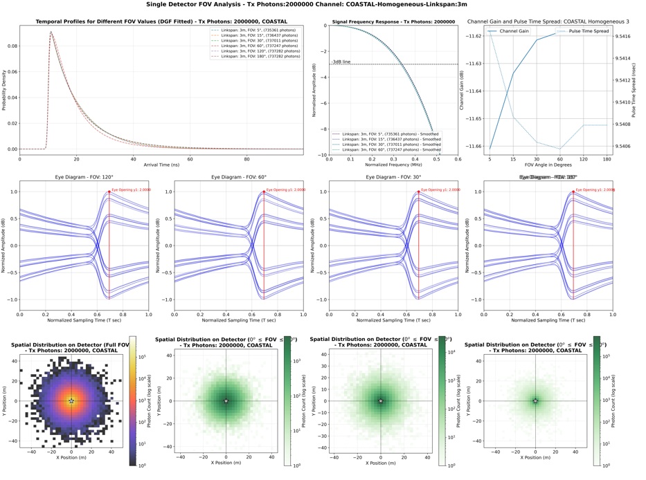
The SISO report engine generates a layout of subplots with 6 rows by 4 columns (see Figure 2a and Figure 2b on the left). In some cases, you may notice that two columns are merged to improve plot resolution. The plots are saved at 450 DPI resolution. Each subplot corresponds to a specific data file in either Excel or JSON format. This means that once you download the numerical data, you can perform your own analysis on your machine. If you need assistance, feel free to reach out via email—we're here to help!
Each row represents specific features related to the temporal and spatial distribution of the received photons. The last two rows display statistics from the Double-Gamma Function (DGF) curve-fitting process. The temporal and spatial distributions are plotted as functions of the field-of-view (FOV) angle, spanning 180 degrees. Additionally, the temporal subplots are mapped into the frequency domain. Further details for each plot are provided in the table below.
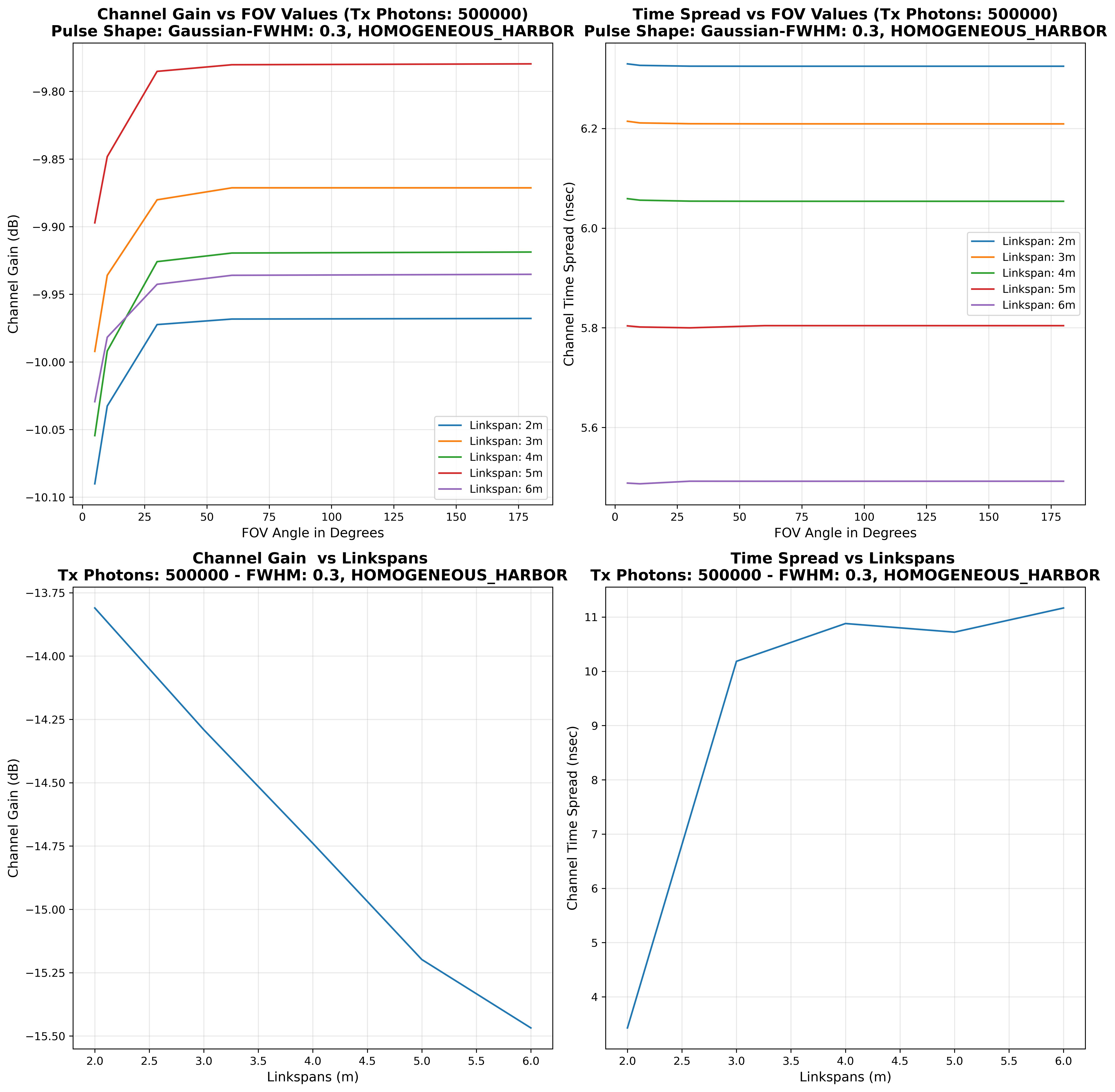
When you select more than four link spans per run, the SISO report engine generates an additional collective plot. This plot displays channel gain and pulse time spread versus link span at each field of view (FOV), with a minimum of five FOVs per set. As a result, there will be four additional subplots.
Subplots in Figure (2a)
- First Row: The Temporal Profile at each FOV
- First two columns:The temporal profile at each selected FOV angles (MCS and DGF fitted data)
- Third column:The Frequency response at each selected FOV angles (for the DGF fitted data) with -3dB line
- Forth column:Channel Gain and Pulse Time Spread at each selected FOV angles (for the DGF fitted data)
- Second Row: Eye Diagrams
- First column:FOV = 180 degrees
- Second column:FOV = 120 degrees
- Third column:FOV = 30 degrees
- Fourth column:FOV = 10 degrees
- Third Row: The spatial (x,y) profile
- First column:FOV = 180 degrees
- Second column:FOV = 120 degrees
- Third column:FOV = 30 degrees
- Fourth column:FOV = 10 degrees
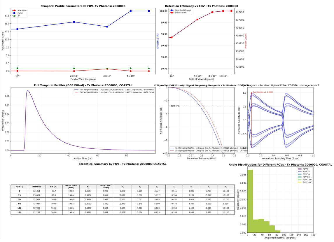
Subplots in Figure (2b)
- Fourth Row:
- First two columns:The Temporal profile parameters (Pulse rise time, FWHM, R2) vs FOV
- Third column:Detection efficiency vs FOV
- Forth column:Empty (for future implementation)
- Fifth Row: Full Temporal Profile
- First two columns:Temporal Profile
- Third column:Frequency Response with -3dB line
- Forth column:Eye Diagrams with Q-line
- Sixth Row: Plotting Statistics
- First three columns:DGF curve fitting parameters and temporal profile parameters
- Forth column:Received photons vs FOV angles
Subplots in Figure (3)
- First Row: Channel Gain and Received Pulse Time Spread vs FOV
- First column:Channel Gain vs FOV for all linkspans
- Second column:Pulse Time Spread vs FOV for all linkspans
- Second Row: Channel Gain and Received Pulse Time Spread vs Linkspans
- First column:Channel Gain vs Linkspans
- Second column:Pulse Time Spread vs Linkspans
Single Input Multi Output - (SIMO)
The SIMO service assists scientific and engineering teams in exploring various use cases by analysing different sets of Prameters. This process helps them identify the optimal features needed to design and build efficient and reliable optical system applications, such as IoT devices, air and underwater drones, and communication systems. As a result, the MCST enables the research team to evaluate potential risk limits before assembling the experimental setup, ultimately saving both time and money.
The SIMO MCST provides the research team with an opportunity to develop an optical receiver that is more tolerant to impairments affecting line-of-sight (LOS) alignment. Additionally, Quadrant and Qantant detectors are utilized to align a network of underwater IoT devices through a management station.
SIMO Prameters:
Transmitter Prameters
- Number of photons.The allowed range of number of photons in the current version is between 200K to 2M.
- Laser/LED wavelength: Blue (450 nm), Green I (488 nm), and Green II (518 nm)
- Baud Rate (GBps): The allowed range of the Gbps in this version is between 1G to 100G.
- Optical source shape: Three types are avialable in this version (1) Gaussian, (2) Rect, and (3) Point Source.
- Pulse width at Half Maxima (PWHM): The PWHM's range is between 0.1 to 0.6.
- Extiniction Ratio: The avialable range is between 1.5 to 2.5.
Propagation Channel Prameters
- Channel Medium Randomness Mode:There are two modes to select from: (1) Homogenous, and (2) InHomogeneous
- Laser/LED wavelength: Blue (450 nm), Green I (488 nm), and Green II (518 nm)
- Seawater Type: In this version the MCST application offers four types of seawater: (1) Clear, (2) Coastal, (3) Harbour, and (4) Torbid
- Linkspan SetMCST application excepts one or more linkspan values (in m) per run.
- Anisotropy Factor (g)The factor value could be between 0.1 and 1.0. The g factor represents the average value of the scattering angle cos.
Based on your selections of parameters the system compute the peak and average power of the optical source.
The volume of data and diagram files in SIMO reports is influenced by the number of use cases integrated into the attribute settings. It is highly advisable to begin with a simple use case and then gradually expand its scope.
Output Data and Diagram Files:
The volume of data and diagram files in SIMO reports is influenced by the number of use cases integrated into the attribute settings. It is highly advisable to begin with a simple use case and then gradually expand its scope.
The SIMO report engine generates a layout of subplots with 3 rows by 2 columns (see the image on the left). In some cases, you may notice that two columns are merged to improve plot resolution. The plots are saved at 450 DPI resolution. Each subplot corresponds to a specific data file in either Excel or JSON format. This means that once you download the numerical data, you can perform your own analysis on your machine. If you need assistance, feel free to reach out via email—we're here to help!
Each row represents specific features related to the temporal and spatial distribution of the received photons. The last two rows display statistics from the Double-Gamma Function (DGF) curve-fitting process. The temporal and spatial distributions are plotted as functions of the field-of-view (FOV) angle, spanning 180 degrees. Additionally, the temporal subplots are mapped into the frequency domain. Further details for each plot are provided in the table below.
When you select more than four link spans per run, the SIMO report engine generates an additional collective plot. This plot displays channel gain and pulse time spread versus link span at each field of view (FOV), with a minimum of five FOVs per set. As a result, there will be four additional subplots.
Figure 7a-Spatial Distribution Over each Quadrant Sector
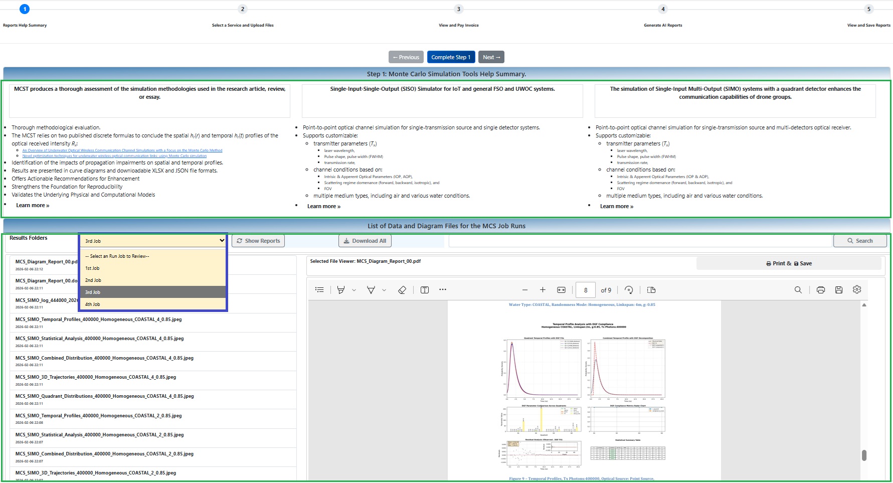
Viewing and Downloading Reports
Once your report(s) are generated in step (4), you can access them in step (5): "View Save Reports" section.
By following this structured journey, you can leverage AI to enhance the quality, rigour, and clarity of your academic research before submission.
- File Viewer: This section displays a list of all your saved reports, organized by the original uploaded file.
- Report Formats: You will find your reports in various formats, including:
- XLSX (Primarily for spatial and temporal received pulse profiles (1) (x,y,z,t) for each FOV angle, (2) (x,y,z,t) for full recieved pulse profile, e.g., Research_Literature_Survey_list_2025-10-10-02_01.xlsx)
- JSON (Primarily for single, e.g., Research_Literature_Survey_list_2025-10-10-02_01.xlsx)
- JPEG (Primarily for all generated diagrams (PDI=450), e.g., Research_Literature_Survey_list_2025-10-10-02_01.xlsx)
- TXT (log files)
- Navigation: At Step 1; you can view, download, and manage all your MCST session runs' reports from this centralized location.
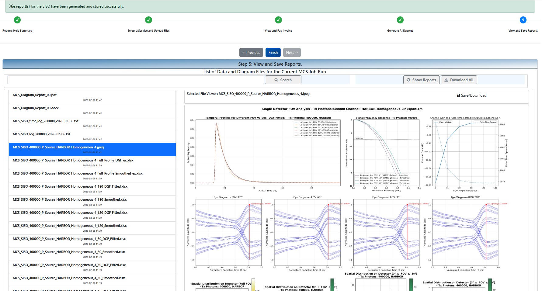
Figure 8 - Report List, View selected Report, and Download Files
Step by Step Guide
The MCST application has been constructed in a wizard-style dialogue. The application's vertical menu item is located on the left-hand side of the main screen.
Step 1: Reports Help Summary
Once you press the Academic AI Review menu item, you will land on the screen of the first step of the wizard. This step is a summary of help for the three AI services. Each summary service's help includes a list of benefits and a "Learn more" anchor button that takes you to the complete help for that service.
MCST Step 1: MCST Main Page
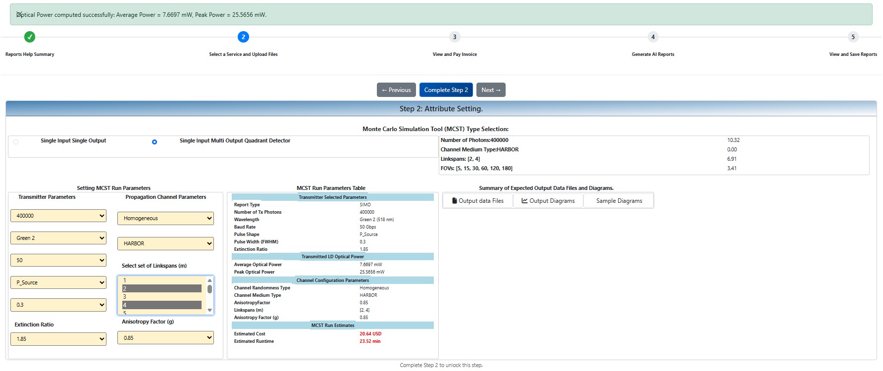
Step 2: Attribute Setting
Once you are familiarized with the underlying benefits of each service, you can press the complete step button. Now, you will be in a position to select the most needed academic service.
Service selection is via a mutually exclusive three-radio-button selection. Once you select a service, the MCST app lets you upload the required number of PDF files and sizes for that service.
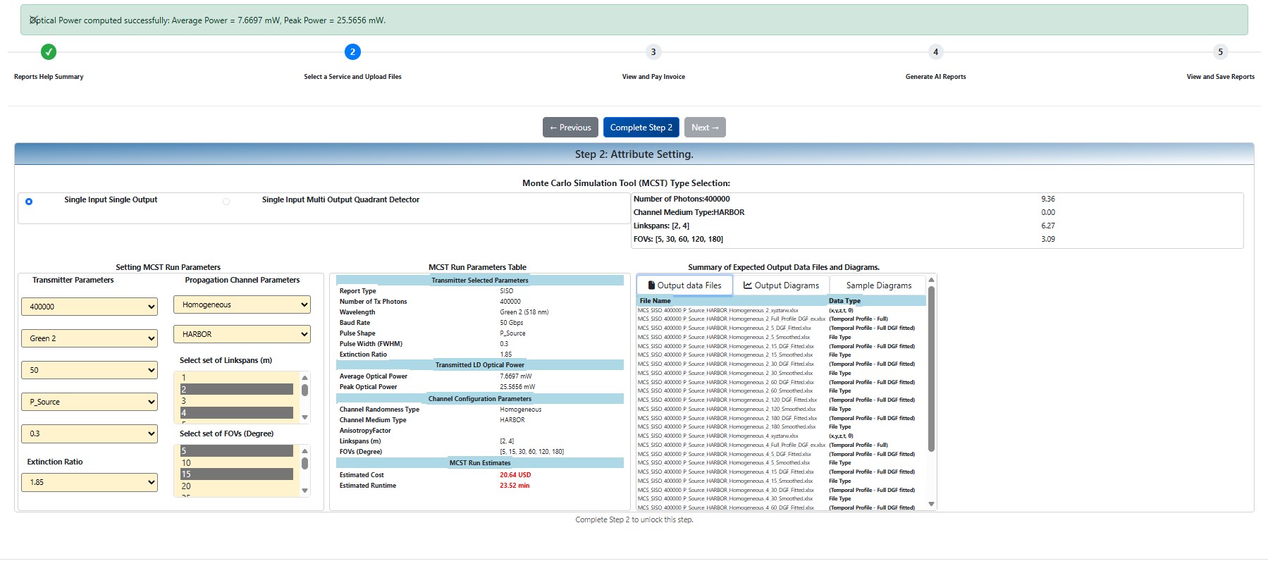
MCST Step 2: MCST Wizard Second Step - Select attribute values for MCS run
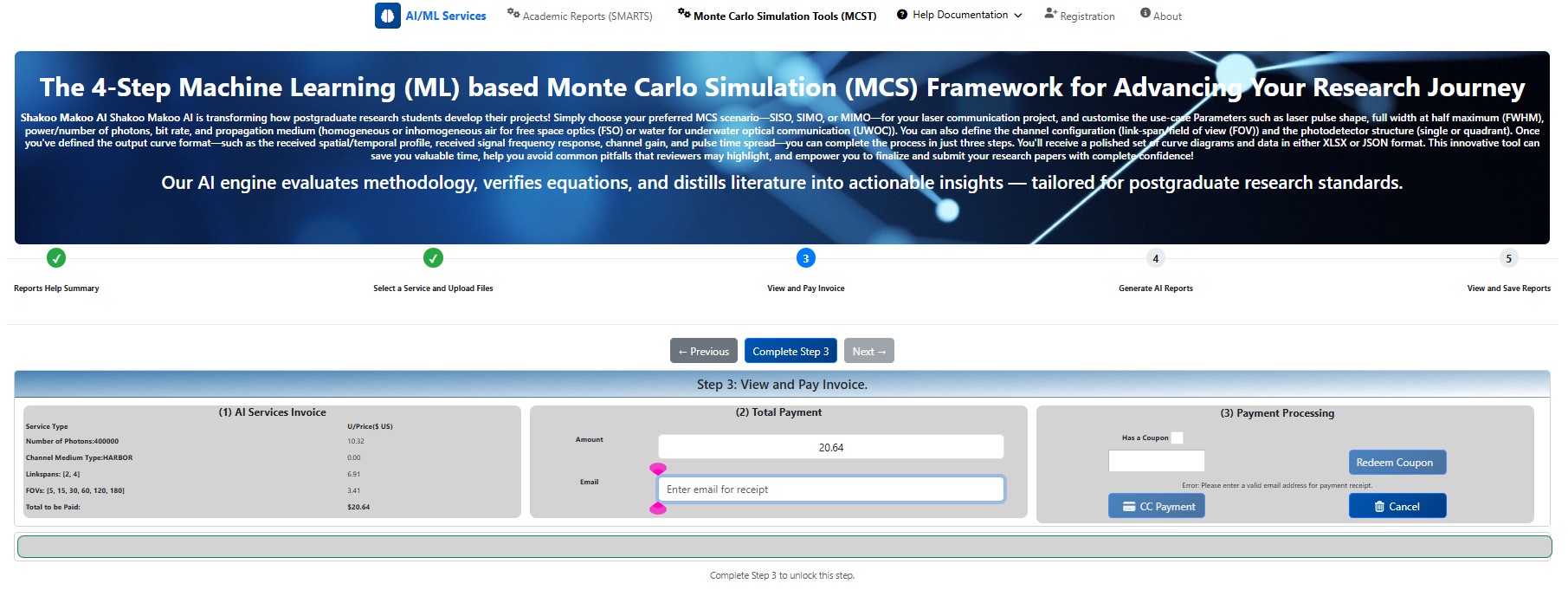
Step 3: View and Pay Invoice
Review the invoice and enter card details to process payment.
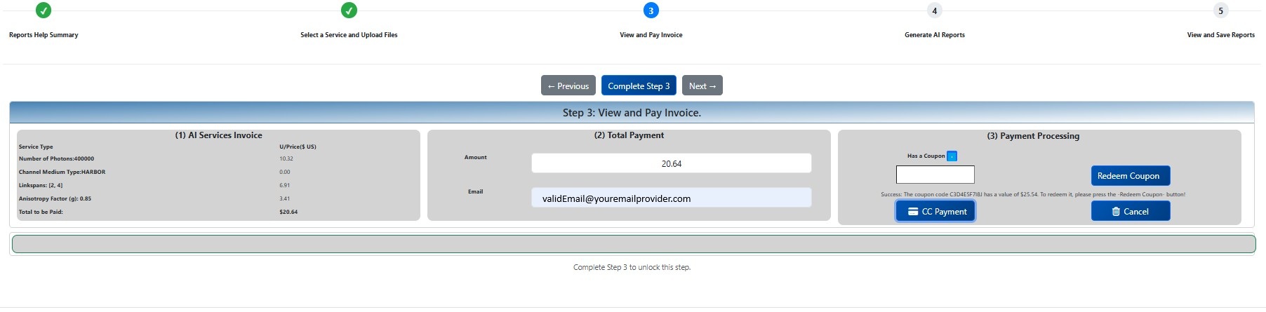
- (a) Reviewing the Invoice: You can find the invoice in the top-left corner of the screen. It displays the selected AI services for each file, along with their corresponding costs in USD. The total amount due is shown at the bottom of the item list on the invoice. If you are not satisfied with your selection of AI services or the costs, you have the option to cancel. To cancel, click the "Cancel" button. The application will then return you to the first step.
MCST Step 3(a): View and Pay Invoice - Reviewing the Invoice
- (b) Entering an Eamil: To proceed, please enter a valid email address linked to your credit card (CC). After entering the email, the "Has a Coupon" checkbox and Coupon Code field will become active.
MCST Step 3(b): View and Pay Invoice - Entering the Email
- (c) Entering the Coupon Code: Once you provide the email, the "Has a Coupon" checkbox and the Coupon Code field will become active. If you have a coupon code, please enter it; if not, you can proceed directly to the credit card (CC) payment stage.
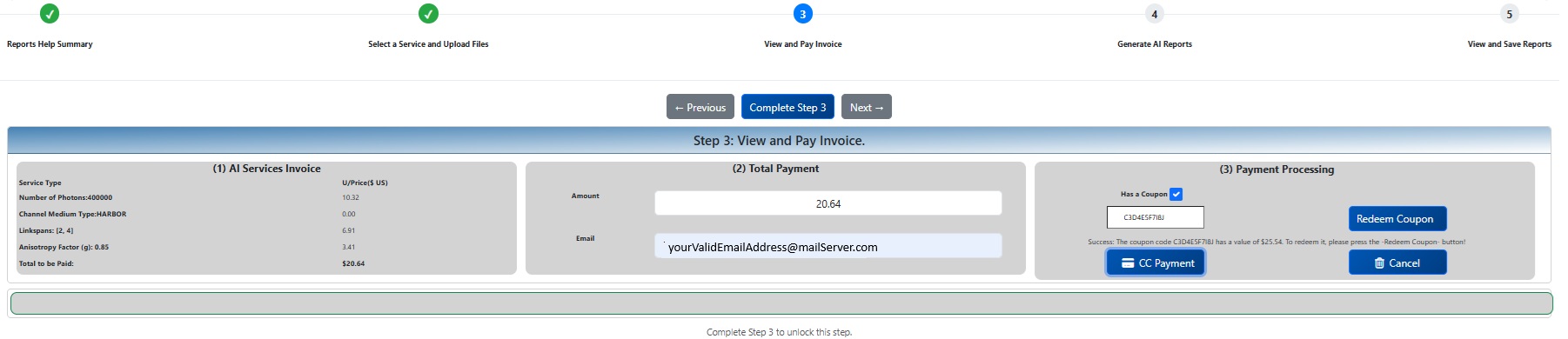
MCST Step 3(c): View and Pay Invoice - Has a Coupon and Entering the Coupon Code
- (d) Redeeming the Coupon or Credit Card Payment: If you have an active coupon with a valid balance, the application will calculate the final amount due. If the total invoice amount is zero, the "CC Payment" button will be inactive, indicating that you can proceed to the fourth step (Monte Carlo Simulation and reports generation). If the total is greater than zero, you will need to click the "CC Payment" button to move on to the next step.
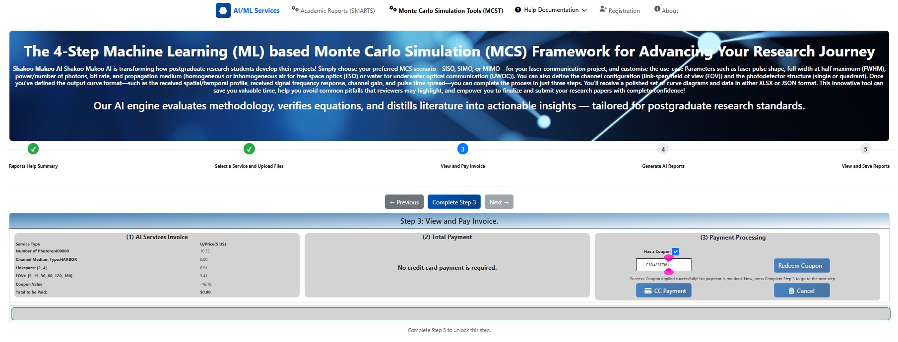
MCST Step 3(d): View and Pay Invoice - Redeeming the Coupon or CC Payment
Step 4: Run Monte Carlo Simluation and Generate AI Reports
You're all set to dive into the Monte Carlo Simulation (MCS) and generate insightful AI reports! The step screen features three informative sections to guide you.
| Section | Contents | Purpose |
|---|---|---|
| (a) MCS and AI Reports Generation | The list of MCST attributes | Executing the MCS run and generating the AI reports. |
| (b) The Progress Report | Report generation progress report | We want to keep you informed about the background processing and what’s happening. |
| (c) The real-time progress indicator | Real-time timer | Progress timeline. |
Table 2. The Sections of the Fourth Step
Note:
- No report attributes are required to generate the MCST reports.
- Cancelling the MCST run at this stage will not entitle you to a refund.
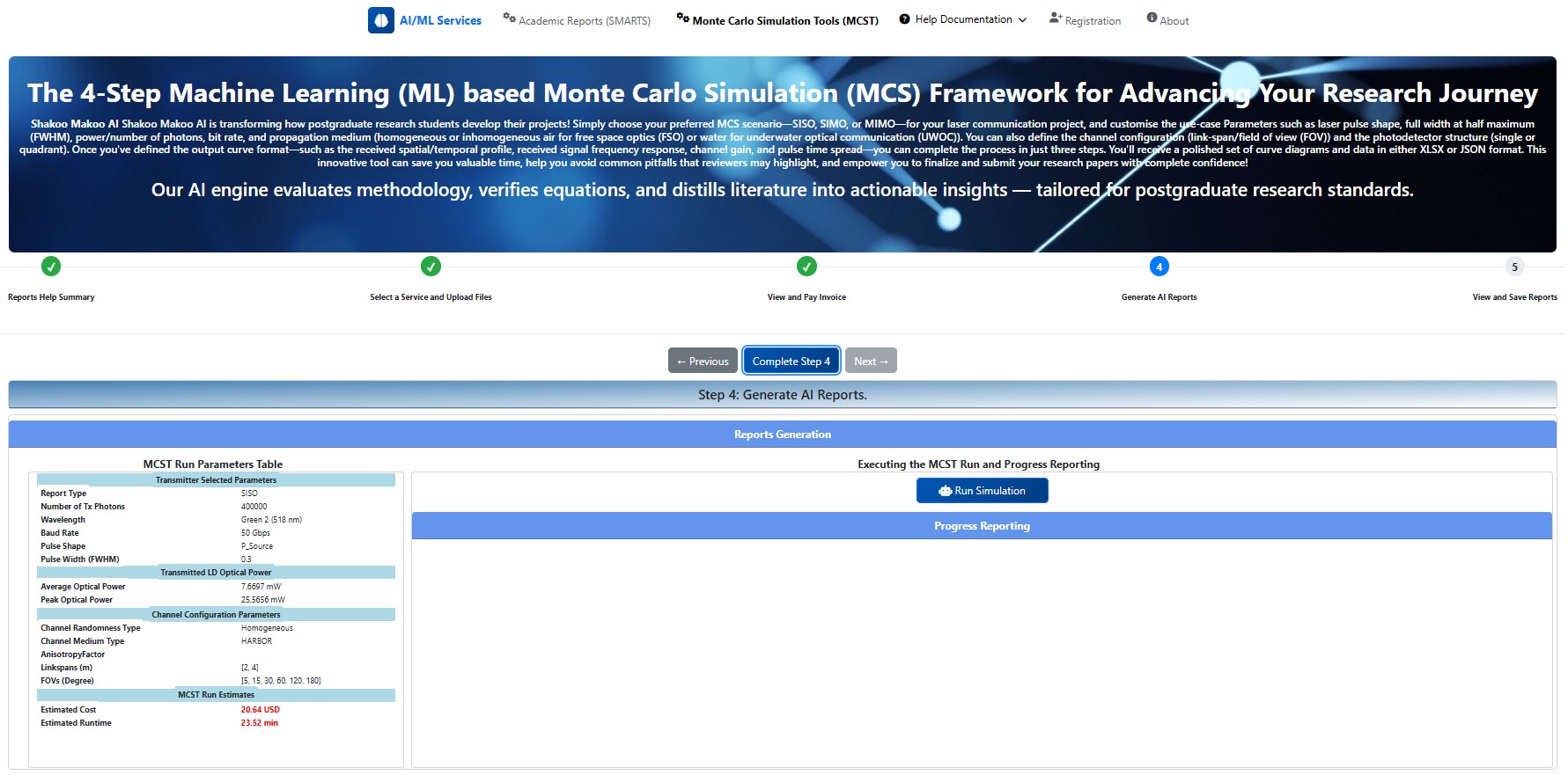
MCST Step 4: - MCST Wizard Fourth Step - Run MCS and Generate AI Reports
Step 5: View and Download Reports
Now you are ready to view the generated AI report list and selectively view individual reports. The screen of this wizard step includes two sections:
| Section | Contents | Purpose |
|---|---|---|
| (a) The report list (on the LHS of the screen) |
|
The MCST AI engine's generated reports for the selected services are displayed in this list, all from a single connection session. |
| (b) Report Viewer |
|
To view, save, and print the report. |
Table 3. The Sections of the Fifth Step
The list contains three file extensions: JSON, XLSX, and TXT.
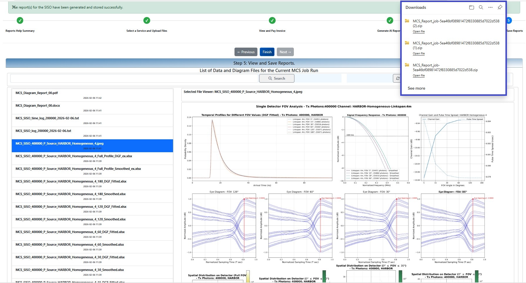
MCST Step 5 - MCST Wizard Fifth Step - View and Download Reports